▷ Coordinate Axis Systems

Ordered pairs of numbers

To start with this post of the cartesian coordinate system or mostly known as the Cartesian plane, let’s suppose that we have 3 electric type pokémon (Luxray, Raikou and Manectric) and 2 fire type pokémon (Charizard and Cyndaqüil), and the conditions of the gym where we will fight is that we can only choose 1 pair to fight but it can only be 1 pokémon of each type. So you, as a pokémon master, decide to give each pokémon a number:

\begin{array}{l l l} \text{Electric} & \quad & \text{Fire} \\ \text{1. Luxray} & & \text{1. Charizard} \\ \text{2. Raikou} & & \text{2. Cyndaqüil} \\ \text{3. Manetric} & & \end{array}

And you make a list to know the combinations you can make for the battle:

\begin{array}{c} 1, 1 \\ 1, 2\\ 2, 1 \\ 2, 2 \\ 3, 1 \\ 3, 2 \end{array}

I tell you that the first number of each combination belongs to the electric-type pokémon and the second number belongs to the fire-type pokémon. If we flip the order of each combination of numbers, we will supposedly have 2 electric-type pokémon and 3 fire-type pokémon, but we know that this is not true! So the order of each pair of combinations is important! With this knowledge, we can write the following:

$\left ( a, b \right) \neq \left( b,a \right)$

$\left( a,b \right) = \left( b,a \right) \text{ if and only if } a = b$

Points in the Cartesian plane

One of the many applications of the pairs of points is the location of these points in the coordinate axes in a Cartesian plane. I’m sure many of us know the classic naval battle game and remember that to locate the ships we had to say a coordinate, and what satisfaction we got when we found our friend’s boat.

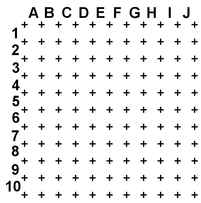
Figure 1. An example board from the Naval Battle game

Imagining an infinite board, we can only use positive and negative numbers, such as using an array of two number lines that intersect at the origin, which is the point $(0, 0)$ where the two lines intersect. Also, each line has a name, the horizontal line is the abscissa line and the vertical line is the ordinate line and each one has a letter, $x$ is the axis of the abscissa and $y$ is the axis of the ordinate. Let’s look at the following coordinate axis system.

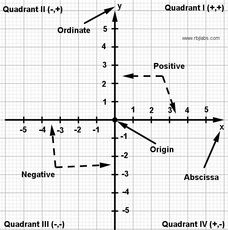
Figure 2. Cartesian Coordinate System

Thus we can conclude that the points are always represented as follows:

$(\text{abscissa}, \text{ordinate})$

And as visualized in the previous image, the coordinate axes system is made up of 4 regions, numbered from one to four in the order as shown in figure 2.

Geometric locations on a Cartesian plane

For analytical geometry topics, the following problems can be presented:

Find the locus (geometric place) that represents an equation and
Find the equation that represents a geometric place.

Thus we can say that a locus is a region of space delimited by a set of points that share a particular mathematical relationship.

For the loci (plural o geometric place), we will see how to solve problems with the analytical part and with the geometric part:

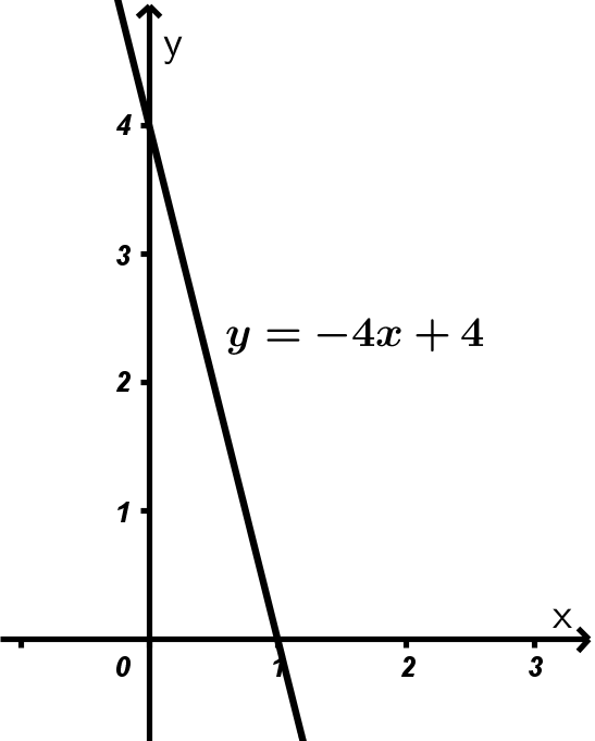
Example 1. Using the equation $y = -4x + 4$ , represent the:

Analytical part of the locus

At first glance it can be understood that it is an equation of the first degree and therefore it is linear, which means that it represents a line. To solve the analytical part we will perform a tabulation using any two points since the given equation is a straight line.

\begin{array}{| c | c |} \hline \ x\ &\ y\ \\ \hline 0 & 4 \\ \hline 1 & 0 \\ \hline \end{array}

With that we already have the analytical part of the equation $y = -4x + 4$

Geometric part of locus

For the geometric part, what we do is draw a straight line that passes through the points that we find in the analytical part.

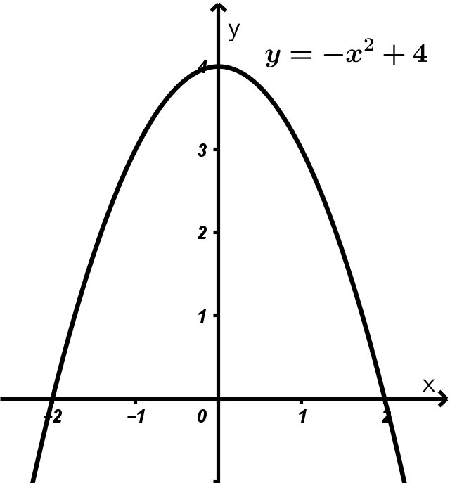
Figure 3. Geometric part of example 1

Example 2. Using the equation $y = -x^{2} + 4$ , represent the:

Analytical part of the locus

What we can see is that the equation is second order, so it represents a parabola, so for the analytical part, we will take various values for the $x$ axis and simply substitute them in the equation of this example, observe the values that it takes if we tabulate them:

\begin{array}{| c | c |} \hline \ x\ &\ y\ \\ \hline -2 & 0 \\ \hline -1 & 3 \\ \hline 0 & 4 \\ \hline 1 & 3 \\ \hline 2 & 0 \\ \hline \end{array}

Geometric part of locus

For the geometric part, what we do is place each of the points of the analytical part and draw the union of the points until we obtain the following ellipse:

Figure 4. Geometric part of the example 2.

Rectilinear segments

The rectilinear segment is a portion of the line between two points. You can have a line, you take two points and the segment that is between those two points is your rectilinear segment.

Since the line has an infinite distance, the rectilinear segment does have a distance that can be calculated (a finite distance). To calculate the distance of a rectilinear segment, we use the following formula:

$d = \sqrt{\left( x_{2} - x_{1} \right)^{2} +\left( y_{2} - y_{1} \right)^{2}}$

Let me tell you that it does not matter if you put the values of the first point or the second point first, the result will be the same, I explain it better with the following equation:

$d = \sqrt{\left( x_{2} - x_{1} \right)^{2} +\left( y_{2} - y_{1} \right)^{2}} =\sqrt{\left( x_{1} - x_{2} \right)^{2} +\left( y_{1} - y_{2} \right)^{2}}$

Distance between two points on the Cartesian plane

Let’s look at a quick example of the distance between two points of rectilinear segments:

Example. Find the distance between the points $A(1,1)$ and $B(6,3)$ .

We draw the points to have a better visualization of the exercise:

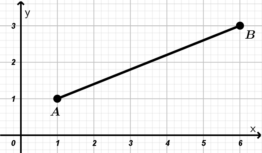
Figure 5. Example of the rectilinear segment

Using the distance between two points formula, we simply substitute their values, remember that we can take the point $A$ as $(x_{1}, y_{1})$ and $B$ as $(x_{2}, y_{2})$ or vice versa:

$d= \sqrt{\left( x_{2} - x_{1} \right)^{2} +\left( y_{2} - y_{1} \right)^{2}} =$

$\sqrt{\left(1 - 6 \right)^{2} +\left(1 - 3 \right)^{2}} = \sqrt{\left(6-1 \right)^{2} +\left(3 - 1 \right)^{2}}$

$=\sqrt{29}$

The distance between the points $A$ and $B$ is equal to $\sqrt{29}$ which is approximately $5.385$ units.

Midpoint of a segment in the Cartesian plane

When we want to calculate the midpoint of a given segment, we can use the following formulas to calculate that point between the ends of the segment:

$x_{m} = \cfrac{x_{1} + x_{2}}{2} \quad y_{m} = \cfrac{y_{1} + y_{2}}{2}$

Example. Calculate the midpoint of the segment comprised by the points $A(1,3)$ and $B(5,-1)$

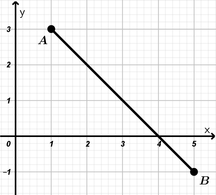
Figure 6. Geometric representation of the points $A$ y $B$

To calculate the midpoint we simply apply the aforementioned formulas:

$x_{m} = \cfrac{1 + 5}{2} \quad y_{m} = \cfrac{3 + (-1)}{2}$

$x_{m} = 3 \quad y_{m} = 1$

We conclude that the midpoint between the points $A$ and $B$ is $(3,1)$ .

Lines in the Cartesian plane

In this section we have to talk about two very important topics of lines, which are the angle of inclination and the slope of the lines.

What we have to know is that there is an indestructible friendship bond between the slope and the angle of inclination, look at the figure 7, the slope is any line, ray or segment that is inclined (see blue dotted line in the figure 7) and the angle of inclination is the elevation of said trace:

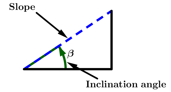
Figure 7. Representation of slope and inclination angle.

With figure 7, we can write the formula for the friendship between the slope and the angle of inclination:

$m = \tan \beta \qquad \beta = \tan^{-1} m$

Where $m$ means slope.

For these exercises we always use degrees, so make sure your calculator is in degrees because if not, you will suffer.

For the calculation of the slope there is a very powerful formula that I am going to leave you below, you can use it as long as you have two points:

$m = \cfrac{y_{2} - y_{1}}{x_{2} - x_{1}}$

The slope of the lines is always the value that multiplies the term $x$ :

$y = mx + b$

Where $b$ is any constant.

Remember that for these particular cases, the slope and the inclination angle will always be measured with respect to the horizontal or line parallel to the abscissa axis.

Next we will put some very simple examples on the calculation of the slope and the inclination angle. If you want us to put more examples, leave it in the comments.

Example 1. Calculate the slope of the following line

Figure 8.

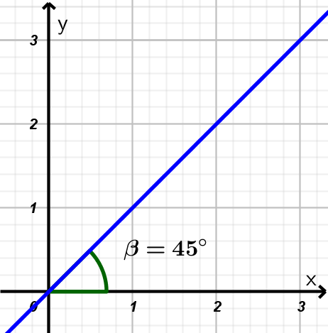
We have almost solved this exercise because they are giving us the angle of inclination of the line, simply what we have to do is substitute in the formula:

$m = \tan 45°$

Using a calculator and making sure that it is in degrees, we will have as a result that the slope of the line $y = x$ is equal to $1$ .

Example 2. Calculate the angle of inclination of the following line.

Figure 9.

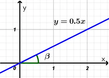
This exercise takes a little more thinking to solve. We can do two things:

Tabulate two points to calculate the slope of the line, or
If we realize this, we will observe that since they give us the equation of the line, they already give us the same slope which is $0.5$ .

So before going to make your tabulation table, the best thing is to analyze the data that they are giving us and realize that they already saved us the work of calculating the slope, so we simply substitute in the formula of the indestructible friendship of the slope and the angle of inclination (always using the calculator in degrees):

$\beta = \tan^{-1} m \longrightarrow \beta = \tan^{-1} (0.5) \approx 26.56$

So the angle of inclination of the line $y=0.5x$ is $26.56°$

Thank you for being in this moment with us : )